Average Number of Years Lost For People Who Died of Coronavirus in France

We illustrate the use of the package by estimating the average number of years by which people’s lives are shortened due to coronavirus. Using data from here that gives us the distribution of ages of people who died from COVID-19 in France, we find that people’s lives are shortened by about 9 years on average. And that this number has not changed through the crisis.

import matplotlib.ticker as ticker
import pandas as pd
import seaborn as sns

from lost_years import lost_years_who

sns.set(style="darkgrid")

Prepare example input in DataFrame

Please look at country codes here:- https://www.lifetable.de/cgi-bin/country_codes.php

df = pd.read_csv("data/covid-cedc-quot.csv", delimiter=";")
list(df)

['reg', 'cl_age90', 'Dc_Elec_Covid_cum', 'jour']

df["jour"].head()

0    2020-03-06
1    2020-03-07
2    2020-03-08
3    2020-03-09
4    2020-03-10
Name: jour, dtype: object

df.columns = ["reg", "age", "n_deaths", "date"]
df.drop(df.loc[df.age == 0].index, inplace=True)
df

	reg	age	n_deaths	date
73	1	9	0	2020-03-06
74	1	9	0	2020-03-07
75	1	9	0	2020-03-08
76	1	9	0	2020-03-09
77	1	9	0	2020-03-10
...	...	...	...	...
16055	94	90	0	2020-05-13
16056	94	90	0	2020-05-14
16057	94	90	0	2020-05-15
16058	94	90	0	2020-05-16
16059	94	90	0	2020-05-17

14600 rows × 4 columns

df2 = df.groupby(["date", "age"]).agg({"n_deaths": sum})
df2

		n_deaths
date	age
2020-03-06	9	0
	19	0
	29	0
	39	0
	49	0
...	...	...
2020-05-17	59	400
	69	1021
	79	2060
	89	3966
	90	2645

730 rows × 1 columns

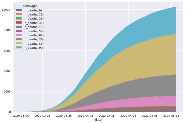
df2.unstack().plot(kind="area", stacked=True, figsize=(12, 8))

<matplotlib.axes._subplots.AxesSubplot at 0x7f30566eec10>

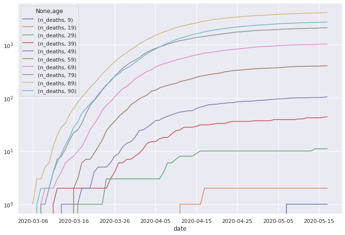
df2.unstack().plot(logy=True, figsize=(12, 8))

<matplotlib.axes._subplots.AxesSubplot at 0x7f3053d51090>

df2.reset_index(inplace=True)
df2

	date	age	n_deaths
0	2020-03-06	9	0
1	2020-03-06	19	0
2	2020-03-06	29	0
3	2020-03-06	39	0
4	2020-03-06	49	0
...	...	...	...
725	2020-05-17	59	400
726	2020-05-17	69	1021
727	2020-05-17	79	2060
728	2020-05-17	89	3966
729	2020-05-17	90	2645

730 rows × 3 columns

df2["year"] = 2020
df2["country"] = "FRA"
df2["sex"] = "M"

df2

	date	age	n_deaths	year	country	sex
0	2020-03-06	9	0	2020	FRA	M
1	2020-03-06	19	0	2020	FRA	M
2	2020-03-06	29	0	2020	FRA	M
3	2020-03-06	39	0	2020	FRA	M
4	2020-03-06	49	0	2020	FRA	M
...	...	...	...	...	...	...
725	2020-05-17	59	400	2020	FRA	M
726	2020-05-17	69	1021	2020	FRA	M
727	2020-05-17	79	2060	2020	FRA	M
728	2020-05-17	89	3966	2020	FRA	M
729	2020-05-17	90	2645	2020	FRA	M

730 rows × 6 columns

fr_ldf = lost_years_who(
    df2, {"age": "age", "country": "country", "sex": "sex", "year": "year"}
)
fr_ldf.head()

	date	age	n_deaths	year	country	sex	who_age	who_country	who_life_expectancy	who_sex	who_year
0	2020-03-06	9	0	2020	FRA	M	10	FRA	70.5	MLE	2016
1	2020-03-06	19	0	2020	FRA	M	20	FRA	60.6	MLE	2016
2	2020-03-06	29	0	2020	FRA	M	30	FRA	50.9	MLE	2016
3	2020-03-06	39	0	2020	FRA	M	40	FRA	41.3	MLE	2016
4	2020-03-06	49	0	2020	FRA	M	50	FRA	32.1	MLE	2016

gldf = fr_ldf.groupby(["date", "age", "who_life_expectancy"]).agg({"n_deaths": sum})
gldf

			n_deaths
date	age	who_life_expectancy
2020-03-06	9	70.5	0
	19	60.6	0
	29	50.9	0
	39	41.3	0
	49	32.1	0
...	...	...	...
2020-05-17	59	23.8	400
	69	16.2	1021
	79	9.4	2060
	89	6.7	3966
	90	6.7	2645

730 rows × 1 columns

gldf.reset_index(inplace=True)
gldf

	date	age	who_life_expectancy	n_deaths
0	2020-03-06	9	70.5	0
1	2020-03-06	19	60.6	0
2	2020-03-06	29	50.9	0
3	2020-03-06	39	41.3	0
4	2020-03-06	49	32.1	0
...	...	...	...	...
725	2020-05-17	59	23.8	400
726	2020-05-17	69	16.2	1021
727	2020-05-17	79	9.4	2060
728	2020-05-17	89	6.7	3966
729	2020-05-17	90	6.7	2645

730 rows × 4 columns

gldf["years_lost"] = gldf["who_life_expectancy"] * gldf["n_deaths"]
gldf

	date	age	who_life_expectancy	n_deaths	years_lost
0	2020-03-06	9	70.5	0	0.0
1	2020-03-06	19	60.6	0	0.0
2	2020-03-06	29	50.9	0	0.0
3	2020-03-06	39	41.3	0	0.0
4	2020-03-06	49	32.1	0	0.0
...	...	...	...	...	...
725	2020-05-17	59	23.8	400	9520.0
726	2020-05-17	69	16.2	1021	16540.2
727	2020-05-17	79	9.4	2060	19364.0
728	2020-05-17	89	6.7	3966	26572.2
729	2020-05-17	90	6.7	2645	17721.5

730 rows × 5 columns

gldf2 = gldf.groupby(["date"]).agg({"years_lost": sum})
gldf2

	years_lost
date
2020-03-06	6.7
2020-03-07	26.8
2020-03-08	59.1
2020-03-09	88.7
2020-03-10	104.8
...	...
2020-05-13	93752.9
2020-05-14	94148.7
2020-05-15	94637.7
2020-05-16	95203.9
2020-05-17	95625.1

73 rows × 1 columns

gldf2 = gldf2.join(fr_ldf.groupby(["date"]).agg({"n_deaths": sum}))
gldf2["avg_years_lost"] = gldf2.years_lost / gldf2.n_deaths
gldf2

	years_lost	n_deaths	avg_years_lost
date
2020-03-06	6.7	1	6.700000
2020-03-07	26.8	4	6.700000
2020-03-08	59.1	7	8.442857
2020-03-09	88.7	10	8.870000
2020-03-10	104.8	12	8.733333
...	...	...	...
2020-05-13	93752.9	10064	9.315670
2020-05-14	94148.7	10109	9.313354
2020-05-15	94637.7	10165	9.310152
2020-05-16	95203.9	10217	9.318185
2020-05-17	95625.1	10254	9.325639

73 rows × 3 columns

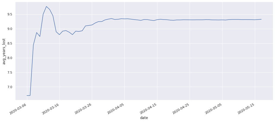
g = sns.relplot(x="date", y="avg_years_lost", kind="line", data=gldf2.reset_index())
g.fig.autofmt_xdate()
g.fig.set_figwidth(16)
g.fig.set_figheight(6)
for ax in g.axes.flatten():
    ax.xaxis.set_major_locator(ticker.MultipleLocator(10))